FreeFlow:用 Latent Flow Matching 估计跨维分子自由能差
FreeFlow:用 Latent Flow Matching 估计跨维分子自由能差
论文:FreeFlow: Latent Flow Matching for Free Energy Difference Estimation
作者:Ege Erdogan, Radoslav Ralev, Mika Rebensburg, Céline Marquet, Leon Klein, Hannes Stärk
版本:用户提供的是 ICLR 2025 匿名投稿;具名版本发表于 ICLR 2025 MLMP Workshop
链接:OpenReview submission / Workshop page / Workshop OpenReview
源说明:OpenReview PDF 在本次检索中返回 verification challenge,无法保存并逐页渲染。本文依据官方 PDF 的搜索索引文本精读,并与 ICLR workshop 页面、作者公开页面交叉核对;文中两张图均为依据论文方法与报告数值重新绘制,不是 PDF 原图。检索日期:2026-08-26。
开篇判断:它不是“用神经网络直接预测自由能”
FreeFlow 最容易被误读成一个自由能回归模型。其实它做的是另一件事:先学习怎样把体系 $A$ 的平衡样本搬运到体系 $B$,再把这条搬运路径造成的密度变化写回 free-energy perturbation estimator。
这个区别很关键。网络没有接收一个分子对,然后直接吐出 $\Delta F$;它接收两端 molecular dynamics 产生的坐标样本,用两个 autoencoder 把不同维度的坐标压进同一个 latent space,再用 flow matching 学一条连续 transport。估计阶段仍然要计算物理势能 $U_A$、$U_B$,也仍然依赖统计力学里的指数平均。
论文最有意思的贡献因此不是“flow matching 能做分子”,而是:
当两个分子的原子数不同、坐标维数也不同时,能否不引入 dummy atoms,仍然构造一张带显式 change-of-variables 修正的 targeted FEP map?
FreeFlow 给出的答案是“可以近似做到”。但实验也清楚地划出了边界:它目前更像 transdimensional targeted FEP 的 proof of concept,还不是生产可用的 relative binding free-energy pipeline。
Paper Card
| 项目 | 信息 |
|---|---|
| Paper | FreeFlow: Latent Flow Matching for Free Energy Difference Estimation |
| Authors | Ege Erdogan, Radoslav Ralev, Mika Rebensburg, Céline Marquet, Leon Klein, Hannes Stärk |
| Venue | ICLR 2025 Workshop on Machine Learning Multiscale Processes (MLMP) |
| 核心问题 | 在无需 alchemical intermediate states 和 dummy atoms 的情况下,估计不同维分子体系间的自由能差 |
| 核心组件 | 两个独立 MLP autoencoders、shared latent space、minibatch-OT flow matching、targeted FEP estimator |
| 实验 | Gaussian、alanine dipeptide、六个 ligand subsets 的 solvent leg |
| 公开实现 | 截至 2026-08-26,官方页面及作者公开仓库中未定位到 FreeFlow 代码;论文仅说明将公开代码 |
| 复现判断 | 数学路径清楚,但完整复现受代码、数值配置和精确 evaluation protocol 缺失限制 |
Abstract:这篇论文想替代的是中间态,不是物理模拟本身
自由能差决定了一个体系从状态 $A$ 转到状态 $B$ 的相对热力学稳定性。标准 free-energy perturbation 在理论上很简洁,但当两个状态的高概率区域几乎不重叠时,估计的方差会爆炸。实际计算通常在 $A$ 和 $B$ 之间插入一串 alchemical intermediate states,让相邻分布逐步重叠。
代价也随之而来:每一个中间态都要采样,路径还需要人为设计。对于原子数不同的 ligand transformation,常见实现还会引入不参与真实相互作用的 dummy atoms,以维持状态空间维度一致。
FreeFlow 的思路是把困难转移到 latent space:
- 用 $E_A$ 和 $E_B$ 把两个端点的坐标分布映射到共同 latent space;
- 用 flow matching 学 $Z_A\rightarrow Z_B$ 的连续 transport;
- 用 $D_B$ 把 latent endpoint 解码回体系 $B$;
- 把 encoder、continuous flow、decoder 三段的体积变化全部计入 FEP estimator。
它移除了 alchemical 中间态,却没有移除 endpoint MD、势能计算、ODE 积分和 Jacobian 计算。这个边界贯穿整篇论文。
Motivation:为什么普通 FEP 会失效
对逆温度 $\beta=(k_BT)^{-1}$,两个体系的自由能差是
\[\Delta F=-\beta^{-1}\log\frac{Z_B}{Z_A}.\]Zwanzig free-energy perturbation 把它写成从 $A$ 端采样的指数平均:
\[e^{-\beta\Delta F} =\mathbb E_{x\sim\rho_A} \left[e^{-\beta(U_B(x)-U_A(x))}\right].\]公式没有问题,问题在 sample overlap。假如 $A$ 的典型构象落到 $B$ 的高能区,那么大多数权重都接近 0;真正决定均值的稀有样本在有限轨迹里可能根本不会出现。
Targeted FEP 引入一张 map $f$,先把 $A$ 的样本推到更像 $B$ 的区域:
\[\Psi_F(x)=U_B(f(x))-U_A(x)-\beta^{-1}\log\left|\det J_f(x)\right|.\]如果 $f$ 把 $\rho_A$ 完美搬到 $\rho_B$,理论上每个样本都会给出相同的 work,估计方差降到 0。现实中 map 不会完美,但只要显著改善 overlap,指数平均就可能稳定很多。
传统 normalizing flow map 通常要求输入输出维度相同。这就是 FreeFlow 要突破的技术点:对不同原子数的分子,$J_f$ 不是方阵,普通 determinant 不再成立。
先看结论:实验支持什么,不支持什么
在 Gaussian toy problem 上,FreeFlow 能逼近解析真值,包括 60-D 到 30-D 的跨维 transport;但跨维结果已经出现轻微 bias,作者将其归因于 autoencoder reconstruction 不完全和 off-manifold sample 带来的近似 change of variables。
在 alanine dipeptide 上,论文以二面角 $\phi$ 划分两个 metastable states。五次运行得到
\[\widehat{\Delta F}=19.03\pm1.69\ \text{kJ/mol},\]参考值是 $20.87\ \text{kJ/mol}$。映射后的 pairwise-distance distribution 的确向目标分布靠近,但没有完全重合。
Ligand 实验更复杂,也更应该分开看“排序”和“绝对误差”。
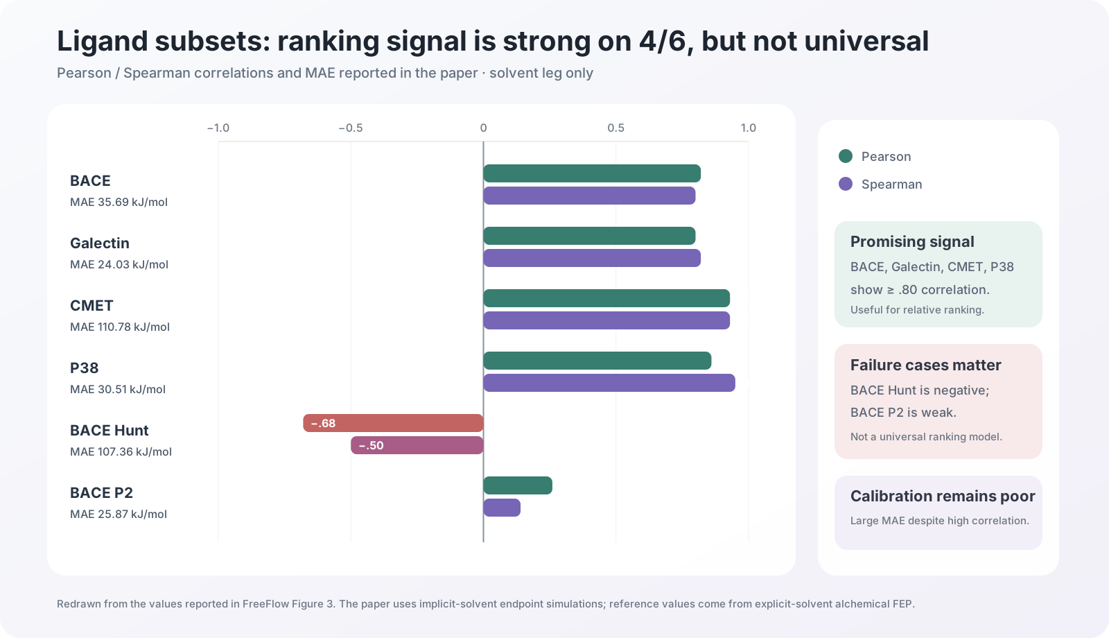
图 1:依据论文 Figure 3 报告数值重绘。BACE、Galectin、CMET、P38 的 Pearson / Spearman correlation 均达到约 0.8 或更高;BACE Hunt 为负相关,BACE P2 相关性很弱。高 correlation 与大 MAE 可以同时出现,因此“能排序”不能被写成“自由能数值准确”。
论文强调 6 个子集中有 4 个取得至少 0.8 左右的 correlation,这个结论成立;但完整读法还应包括另外三点:
- CMET 的 Pearson / Spearman 都是 0.93,MAE 却达到 $110.78\ \text{kJ/mol}$,说明相对趋势和绝对 calibration 是两回事。
- BACE Hunt 的 Pearson 为 -0.68、Spearman 为 -0.50,是方向性的失败,不是小幅退化。
- BACE P2 的 Pearson 只有 0.26、Spearman 只有 0.14,说明方法并不具备稳定的跨 subset 排序能力。
我的判断是:这些结果证明 latent transport 中存在有用的 relative signal,但还不能证明它已经能替代生产级 alchemical FEP。
方法总览:三段映射,一次统计力学修正
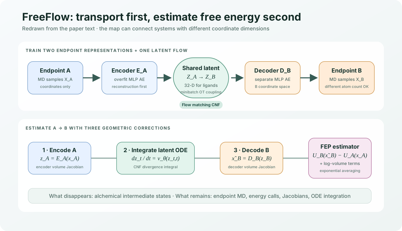
图 2:依据论文方法重绘。训练阶段需要两个 endpoint MD datasets、两个独立 autoencoders 和一个 latent flow。估计阶段从 $A$ 出发,经 encoder、latent ODE、decoder 到达近似的 $B$ 样本,同时累计三段 change-of-variables correction。
FreeFlow 的 end-to-end map 可以写成
\[f(x_A)=D_B\!\left(\operatorname{ODE}\big(E_A(x_A)\big)\right).\]这张 map 由三个性质不同的部件组成:
| 部件 | 输入输出 | 学到什么 | 密度修正 |
|---|---|---|---|
| Encoder $E_A$ | $A$ 坐标 $\rightarrow$ shared latent | 把高维坐标压到低维 manifold coordinate | rectangular Jacobian 的 volume term |
| Latent CNF | $z_A\rightarrow z_B$ | 连续 transport vector field | divergence integral |
| Decoder $D_B$ | shared latent $\rightarrow$ $B$ 坐标 | 把 latent state 展开到 $B$ 的坐标空间 | rectangular Jacobian 的 volume term |
这也是为什么“把两个 autoencoder 接一个 flow”还不是完整方法。真正让它能进入 free-energy estimator 的,是三段密度变化都被显式计算。
第一步:两个独立 autoencoder 只负责建立共同坐标系
体系 $A$ 和 $B$ 分别拥有 $(E_A,D_A)$ 与 $(E_B,D_B)$。输入是展开后的原子坐标,accessed source 中没有把原子类型作为 autoencoder 输入。论文采用简单 MLP,并报告在 alanine 上,相比尝试过的 equivariant GNN,MLP reconstruction error 更低、训练约快 8 倍。
这个设计很反常识,却和任务目标一致。Autoencoder 不是为了在未知分子上泛化,而是要尽量无损地记住当前 endpoint ensemble。作者明确让它们在参与自由能估计的同一批样本上训练到 reconstruction MSE 收敛。
因此,不能把 FreeFlow 解释成一个 transferable molecular representation model。它更像为每一对 endpoint datasets 临时学习两张坐标图。
在 ligand 实验中,无论原始分子有多少个原子,都会编码成 32-D latent。跨维问题于是从“如何让两个坐标空间同维”变成“如何保证 encoder / decoder 的 manifold volume correction 足够准确”。
第二步:用 optimal-transport flow matching 学 latent transport
编码后的分布记为 $Z_A$ 和 $Z_B$。FreeFlow 在 shared latent space 中训练 velocity field $v_\theta(z_t,t)$:
\[\mathcal L_{\mathrm{CFM}}(\theta)= \mathbb E_{t,(x_0,x_1),z_t} \left\|v_\theta(z_t,t)-\big(E_B(x_1)-E_A(x_0)\big)\right\|_2^2.\]这里 $(x_0,x_1)$ 不是随便配对,而是使用 minibatch optimal transport coupling。它希望把相近的 latent endpoints 配在一起,让 transport path 更直、更短,进而降低 ODE 数值误差,也避免轨迹无意义地穿过高自由能区域。
训练完成后,latent state 通过 ODE 演化:
\[\frac{dz_t}{dt}=v_\theta(z_t,t).\]Continuous normalizing flow 的瞬时变量变换公式给出
\[\log\rho(z_1)=\log\rho(z_0)- \int_0^1 \operatorname{tr}\left( \frac{\partial v_\theta(z_t,t)}{\partial z_t} \right)dt.\]右侧的 divergence integral 就是 latent flow 对 log density 的贡献。Flow matching 在这里不只是生成 target-like samples;它还必须提供能够进入 estimator 的密度修正。
第三步:矩形 Jacobian 怎样进入 change of variables
如果 encoder 把 $d_A$ 维坐标压到 $d_z$ 维,$J_E$ 的 determinant 没有定义。论文使用 volume Jacobian:
\[\operatorname{vol}(J)=\sqrt{\det(J^\top J)}.\]根据 Jacobian 是“高维到低维”还是“低维到高维”,相应使用 row-space 或 column-space Gram matrix。把三段 correction 合并,论文定义
\[\begin{aligned} \Psi_F(x_A)=&\ U_B(\tilde x_B)-U_A(x_A)\\ &-\beta^{-1}\left[ -\frac12\log\left|\det(J_{E_A}J_{E_A}^{\top})\right| +\int_0^1\operatorname{tr}\left(\frac{\partial v_\theta}{\partial z_t}\right)dt -\frac12\log\left|\det(J_{D_B}^{\top}J_{D_B})\right| \right], \end{aligned}\]其中 $\tilde x_B=f(x_A)$。最终 estimator 是
\[\widehat{\Delta F} =-\beta^{-1}\log\left[ \frac1N\sum_{i=1}^{N} e^{-\beta\Psi_F(x_A^{(i)})} \right].\]从机制上看,FreeFlow 仍然是 targeted FEP:网络改善 overlap,Jacobian 校正 map 引起的测度变化,指数平均恢复自由能差。
数据全流程:训练和估计分别发生什么
训练阶段
| 顺序 | 输入 | 操作 | 输出 |
|---|---|---|---|
| 1 | 体系 $A$、$B$ 的势能面与初始结构 | 分别运行 endpoint MD | $X_A$、$X_B$ 坐标样本 |
| 2 | 两端坐标样本 | 必要时做 RMSD rotation / translation alignment | 对齐后的 endpoint ensembles |
| 3 | $X_A$、$X_B$ | 独立训练两个 MLP autoencoders | $E_A,D_A,E_B,D_B$ |
| 4 | endpoint samples | 编码到 shared latent | $Z_A,Z_B$ |
| 5 | latent minibatches | optimal-transport coupling + flow matching | vector field $v_\theta$ |
估计阶段
- 从 $A$ 的 endpoint trajectory 取一个 $x_A$。
- 用 $E_A$ 得到 $z_A$,同时计算 encoder volume correction。
- 从 $t=0$ 到 $t=1$ 积分 latent ODE,并累计 divergence。
- 用 $D_B$ 得到 $\tilde x_B$,同时计算 decoder volume correction。
- 调用物理势能函数计算 $U_A(x_A)$ 与 $U_B(\tilde x_B)$。
- 得到 $\Psi_F(x_A)$,对一批样本做 log-domain exponential averaging。
这条路径揭示了它真正节省和没有节省的部分:
| 可能减少 | 仍然需要 |
|---|---|
| 多个 alchemical intermediate states 的 simulation / path design | 两个 endpoint 的充分采样 |
| 不同原子数变换中的 dummy atoms | 每对体系训练 autoencoders 与 latent flow |
| 高维坐标空间中直接学习 invertible map | 势能调用、ODE、divergence 与 Gram determinant |
实验一:Gaussian 是在检查公式,不是分子真实性
论文先用 Gaussian 检查 estimator 能否恢复解析自由能差。
- 同维设置:两个 30-D 零均值 Gaussian,$\Sigma_A=I$,$\Sigma_B=0.5I$。
- 跨维设置:60-D 与 30-D 的零均值、单位协方差 Gaussian。
- 每端 50,000 个样本,latent dimension 为 16。
- Autoencoders 训练 100 epochs,flow 训练 200 epochs。
两种设置都逐渐靠近 ground truth。更值得记住的是跨维设置仍有小的系统偏差:当 autoencoder 不能做到零 reconstruction loss,或者数据点没有严格落在 decoder manifold 上时,使用 volume Jacobian 的 change-of-variables 只是近似成立。
这不是实现小瑕疵,而是方法的核心假设。Gaussian 实验的意义正是把这个 bias 提前暴露出来。
实验二:Alanine 验证同一分子的构象态 transport
Alanine dipeptide 有 32 个原子。论文用二面角 $\phi$ 定义两个状态:
\[A:\ \phi\in[-\pi,0]\cup[2.15,\pi], \qquad B:\ \phi\in(0,2.15).\]实验在 vacuum 中用 OpenMM 模拟 400 ns,time step 为 2 fs,每 500 步保存一次,得到 400,000 个 frames;其中 $A$ 有 371,094 个,$B$ 有 28,906 个。
最终 $19.03\pm1.69\ \text{kJ/mol}$ 与 20.87 kJ/mol reference 的差距不大。这个实验说明,当两端维数相同、势能模型一致、构象空间相对受控时,latent transport 能产生可用的 targeted-FEP correction。
但 pairwise-distance histogram 没有完全对齐,也提醒我们:一个不错的标量 $\Delta F$ 并不自动证明 mapped distribution 已经精确等于 target distribution。
实验三:Ligand 结果的公平读法
这是论文最接近药物发现应用的实验,也最容易被一句“4/6 subsets correlation 超过 0.8”概括过头。
实验协议
- 数据来自 Protein-Ligand Benchmark 的 BACE、Galectin、CMET、P38、BACE Hunt、BACE P2。
- 每个 ligand 单独在水中、300 K 下模拟 400 ns,2 fs 一步,每 200 步保存,得到 1,000,000 个样本。
- FreeFlow 侧使用 implicit GBn2 solvation 和
gaff-2.11。 - 参考
pmx数值来自 explicit-solvent alchemical FEP。 - 每个 ligand 的 autoencoder 训练 500 epochs,latent flow 训练 200 epochs。
- 只计算 solvent leg,没有计算 protein-bound complex leg。
为什么 correlation 高但 MAE 仍然大
如果对一组 transformation 全部加上近似一致的系统偏置,Pearson / Spearman 可能依然很好,但绝对值会整体错位。Implicit solvent、force field 和 explicit-solvent reference 的 protocol mismatch 本身就会造成这种现象。
因此当前表格同时混合了至少三类误差:
- latent map 没有准确匹配目标分布;
- change-of-variables / numerical integration 有偏差;
- learned protocol 与 reference protocol 的势能面不同。
没有同一势能面、同一 endpoint samples、同一计算预算下的 matched baseline,我们不能把全部 MAE 都归因于 FreeFlow,也不能用 correlation 抹掉这些误差。
为什么 solvent leg 不能等同于完整 RBFE
Relative binding free energy 通常需要 thermodynamic cycle 的两条腿:ligand 在溶液中的 transformation,以及 ligand 在 protein complex 中的 transformation。两者相减才得到相对结合自由能。
FreeFlow 这里只展示 solvent leg。Protein environment 会带来更慢的构象重排、更复杂的 overlap 问题和更多受限自由度。因此,论文证明了一个重要部件,而不是完整 drug-discovery workflow。
Ablation 与证据缺口
这篇论文的 mechanism chain 很长:autoencoder reconstruction、latent dimension、OT coupling、flow integration、encoder CoV、decoder CoV、指数权重稳定性都可能决定最后的 $\Delta F$。但 accessible evidence 中没有看到足够系统的 ablation,把这些因素逐一隔离。
尤其缺少下面几组对照:
- 相同 endpoint samples 下,普通 FEP、同维 targeted FEP、dummy-atom alchemical FEP 与 FreeFlow 的 matched-cost 比较。
- 去掉 OT coupling 或改变 latent dimension 后,transport quality、effective sample size 与 $\Delta F$ bias 怎样变化。
- Autoencoder reconstruction error、Gram determinant condition number 与最终自由能误差之间的相关性。
- Exact divergence 与 stochastic trace estimator 的成本 / 精度对比;accessible source 没有给出足够实现细节确认采用哪一种完整配置。
- 用相同 explicit-solvent potential 评估 FreeFlow 与
pmx,把 method error 和 simulation-protocol error 分开。
论文报告 MLP 比 equivariant GNN 在 alanine reconstruction 上误差更低、训练约快 8 倍,这是一条有用的 engineering observation,但还不是整个 FreeFlow estimator 的端到端 ablation。
复现性:真正难的不是把网络搭出来
按论文描述复刻两个 MLP autoencoders 和一个 torchcfm vector field 并不困难。难的是让下列数值环节同时可靠:
1. Exponential averaging 的尾部稳定性
$e^{-\beta\Psi_F}$ 对 outlier 极端敏感。几个异常的小 $\Psi_F$ 就可能支配均值。实现必须使用 log-sum-exp,并报告 effective sample size、weight distribution 和 bootstrap uncertainty,而不能只报一个平均 $\Delta F$。
2. Gram determinant 的病态性
如果 $J_EJ_E^\top$ 或 $J_D^\top J_D$ 接近 rank-deficient,直接 det 会下溢或产生巨大 log correction。更稳妥的实现需要 SVD / Cholesky 条件检查、jitter policy 和 singular-value diagnostics。
3. ODE 与 divergence 的误差耦合
轨迹位置误差影响 $U_B(\tilde x_B)$,divergence 积分误差影响 log density;两者会一起进入指数权重。Solver tolerance、step count 和 trace estimator 都应该进入敏感性分析。
4. Autoencoder manifold 假设
Autoencoder reconstruction loss 低,不等于所有 transported latent states 都会 decode 到数据 manifold 上。Flow 可能经过训练数据没有覆盖的 latent region,此时 volume-Jacobian 公式的实际偏差更难判断。
5. 代码与配置仍不完整
截至检索日期,官方 paper page 和作者公开 repositories 中没有定位到 FreeFlow 代码。论文提到 PyTorch、torchcfm、OpenMM 与 bgmol,但 exact seeds、hardware、runtime、所有 solver / determinant settings 和完整 evaluation scripts 仍无法端到端审计。
如何定位 FreeFlow 的贡献
我会把它放在三个相邻方向的交叉点:
| 方向 | FreeFlow 的关系 |
|---|---|
| Alchemical FEP | 试图用 learned endpoint transport 替代人工中间态与 dummy-atom path |
| Targeted FEP / normalizing flows | 保留 map + Jacobian correction,但把 invertible map 移到 shared latent space |
| Flow matching for molecules | 不只生成构象,还把 CNF divergence 作为自由能 estimator 的一部分 |
它最扎实的新意,是把“不同分子维数不一致”从 alchemical path 设计问题,重新表述成 manifold change-of-variables 问题。
它还没有回答的问题则是:当我们把 endpoint MD、每对 ligand 的模型训练、Jacobian 和 ODE 成本全算进去,在同等误差目标下是否真的比成熟 FEP pipeline 更便宜?论文没有 wall-clock、energy-evaluation count 或 matched-accuracy curve,暂时不能下这个结论。
总结
FreeFlow 给出了一条很干净的机制链:
\[\begin{aligned} \text{endpoint MD} &\rightarrow \text{two autoencoders} \rightarrow \text{shared latent transport}\\ &\rightarrow \text{three CoV corrections} \rightarrow \widehat{\Delta F}. \end{aligned}\]它的价值有三点:
- 允许不同原子数、不同坐标维数的体系在 shared latent space 中对接,不再依赖 dummy atoms。
- Flow matching 不只是 sample generator,而是可计算 density correction 的 continuous transport。
- 在 Gaussian、alanine 和部分 ligand subsets 上展示了可用信号,说明这条路线值得继续研究。
但同样要保留四个限制:
- Autoencoder manifold change of variables 会带来近似 bias。
- Ligand 绝对误差很大,6 个 subsets 中有 2 个排序失败或很弱。
- 实验只覆盖 solvent leg,不能代表完整 RBFE。
- 没有 matched-cost baseline 与公开代码,尚不能证明生产精度或总成本优势。
所以,一句话评价这篇论文:它成功证明了“跨维 latent targeted FEP 可以成立”,但距离“替代成熟自由能计算”仍有一整套数值稳定性、公平基线和完整 thermodynamic-cycle 验证要补。
References
- Ege Erdogan et al. FreeFlow: Latent Flow Matching for Free Energy Difference Estimation. ICLR 2025 submission / MLMP Workshop paper.
- Peter G. Bolhuis et al. Targeted free energy perturbation and equilibrium transport ideas discussed in the paper’s related work.
- Mike Invernizzi et al. OPES reference used by the paper for the alanine-dipeptide free-energy difference.
- Hahn et al. Protein-Ligand Benchmark and
pmxreference calculations used in the ligand experiments.
Recommended citation: Ege Erdogan, Radoslav Ralev, Mika Rebensburg, Céline Marquet, Leon Klein, and Hannes Stärk. FreeFlow: Latent Flow Matching for Free Energy Difference Estimation. ICLR Workshop on Machine Learning Multiscale Processes, 2025.
Download Paper